When Explicit Dynamics Looks Right – But Reality Disagrees

In today’s product development landscape, explicit dynamics simulation is widely used to evaluate impact, drop, crash, forming, and other highly nonlinear transient events before physical prototypes are built. Explicit solvers are designed to handle large deformation, complex contact, stress wave propagation, and material failure with numerical robustness.

Yet many engineering teams still encounter a frustrating reality: a product that performs well in simulation can fail during physical testing.

When this gap appears, the solver is often questioned. Discrepancy typically originates from modeling assumptions, mesh quality, contact definitions, material models, or insufficient validation.

The difference between a visually convincing simulation and a truly predictive model lies in engineering discipline, not in the capabilities of the solver.

1. Choosing Explicit Dynamics for Your Simulation Needs

Explicit dynamics is specifically designed to address engineering problems that traditional methods struggle to handle reliably. These include:

• High-speed and transient events such as drop tests, impacts, crashes, explosions, and shock loading, where stress wave propagation governs the response.
• Severe contact and large deformation, including penetration, fragmentation, crushing, forming, stamping, and machining processes.
• Strong material nonlinearity, such as plasticity, hyperelasticity, damage, fracture, and failure evolution.
• Virtual testing under extreme conditions, enabling early performance assessment and regulatory compliance without excessive physical prototypes.

2. Where Simulation–Test Gaps Commonly Originate

Several recurring factors can cause explicit simulations to appear successful while masking non-physical behavior:

• Mass scaling, when applied without control, can alter inertia and energy transfer. While it is a powerful efficient tool, it must always be validated through energy balance (e.g. added mass percentage) rather than runtime improvements alone.
• Velocity or load scaling can unintentionally introduce dominant inertial effects. Even when final deformation looks reasonable, force levels and failure sequences may no longer represent the physical test.
• Hourglass modes, particularly in reduced integration elements, can generate zero-energy deformation that distorts stresses, strains, and energy balance.
• Poorly shaped elements introduce numerical instability, artificial energy, and unreliable failure predictions.

These issues often remain hidden unless the analyst looks beyond contour plots.

3. Overcoming Common Pitfalls in Explicit Analysis

3.1. Mesh Quality:

Mesh quality remains one of the most underestimated contributors to explicit simulation accuracy.

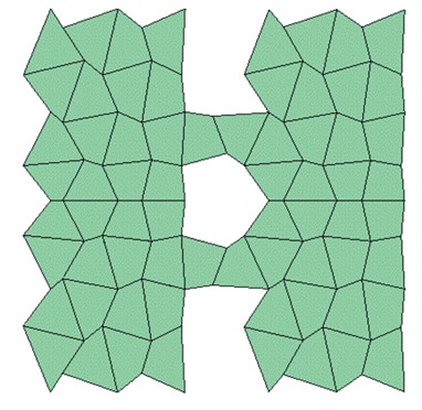
3.1.1. Effects of Poorly Shaped Elements

• Instability and increased solving timescan result from highly distorted or poorly shaped elements, leading to inefficient computation and unreliable results.
• Energy errorscan arise from bad elements, especially if they distort severely under loading, leading to negative volumes or element erosion. This can compromise energy conservation and result in non-physical behavior.
• Small elementscan drastically reduce the critical time step, increasing computational time without necessarily improving accuracy.
• Locking phenomenasuch as shear locking and volumetric locking may occur in linear elements, leading to numerical errors and checkboard modes in results.
• Non-physical artifactssuch as mesh distortion, unrealistic deformation, or spurious failure modes may appear, undermining the validity of simulation results.

Hourglassing can emerge in case of 1-point-integrated hex solid and quad shell elements

Best practice for Explicit Meshing includes:

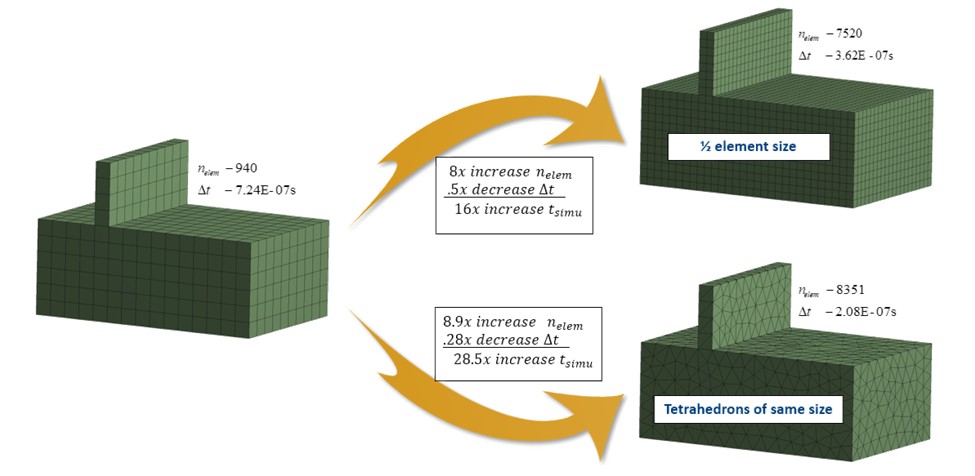
• Prefer hexahedral elementsover tetrahedral elements whenever possible, as they offer better accuracy, and require fewer elements for the same level of fidelity.
• Refine mesh only in critical regions and use coarser mesh elsewhere to optimize computational cost without sacrificing accuracy.
• Avoid poorly shaped or highly distorted elements, as these can cause instability, increase solving time and introduce non-physical artifacts.
• Use simple linear element formulationsfor computational efficiency but be aware of potential hourglass effects in reduced integration elements.
• Element size directly affects the critical time stepdue to the CFL (he Courant-Friedrichs-Lewy) condition; the smallest element determines the stable time step in explicit analysis.

3.2. Energy Conversion:

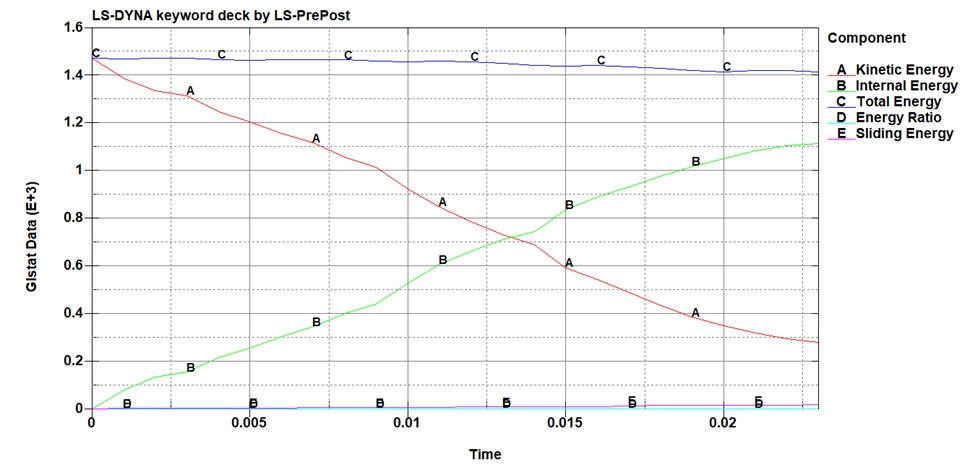
Regardless of the loading regime, energy balance is the primary validation metric in explicit dynamics.

• Always track hourglass energy during the simulation. Excessive hourglass energy compared to internal energy signals mesh or element formulation issues. Hourglass energy shall not exceed 10% of internal energy.

• Monitor kinetic energy in quasi-static simulations; it should remain small relative to internal energy to ensure minimal inertial effects and accurate energy conversion.

• Review energy conservation plots (Energy Summary graphs) for spikes or abnormal trends in hourglass, kinetic, or internal energy, which may indicate non-physical artifacts.

• Use momentum summary graphs and results trackers to observe dynamic stability and detect issues during the solve.

• It is recommended to limit the added mass to less than 5% of the actual mass of each part for dynamic analyses. For quasi-static analyses, up to 20% may be acceptable, depending on the problem being analyzed.

Experienced CAE workflows treat energy histories as first-class results — not as post-processing afterthoughts.

Conclusion:

Explicit dynamics works when engineers respect the fundamentals: mesh quality, material models, contact definition, energy monitoring etc. A predictive model is not about flashy visuals rather it’s about disciplined modeling, controlled assumptions, and continuous validation. That is what turns simulation into a reliable engineering tool.

Author: Ahmed Anwar, Application Engineer, Fluid Codes